Physical Constraints in ML Weather Forecasting
Adding physics to data-driven forecasts

At first glance, the success of ML weather forecasting systems suggests that pattern-matching approaches to forecasting win out over physics-based dynamical approaches. But several teams have recently shown that forecast skill can be improved if physical constraints are built into WF systems. It’s comforting that physics still matters, but surprising that enforcing these constraints improves performance. Neural networks are delicate: enforcing constraints through post-processing or by adding specific model layers could affect model stability and/or performance. But we now have several examples of improved performance when physical constraints are implemented in data-driven systems.
Keeping Variables Within Physical Bounds
The simplest constraint is ensuring that certain variables stay bounded within physical limits. For example, ML systems often predict small negative precipitation rates, which are clearly unphysical. This isn’t surprising, as pure ML forecasts produce statistical estimates and naturally struggle with sharp boundaries.
The latest AIFS update from ECMWF includes a simple fix for this issue by adding an extra layer to the network that zeroes out negative precipitation, and similarly for other variables like fractional cloud cover. This simple constraint substantially improves precipitation skill in AIFS, not just by eliminating negative precipitation values, but also by improving light precipitation (i.e., less drizzle).
The authors showed the improved light rain skill comes about in an interesting way: a negative dry prediction and a drizzle underprediction both produce upward gradients. The network can’t distinguish a genuine physical underprediction (“you should have made more rain”) from an unphysical negative prediction (“there are no negative points in the training set”), and both cases push the network to forecast more light rain. But by zeroing out negative points, this upward bias is removed and the model’s skill is improved.
The variables being bounded are highly localized, so it’s perhaps unsurprising that the model remains stable when the extra layer is added. Implementing sharp bounds also works well with the types of activation functions typically used in neural networks (e.g., ReLU).
But you still might worry that setting the negative values to zero throws away some information – is this a persistently dry regime or is it transitioning to a precipitating state? After digging into the network, the authors show that it retains a record of how dry the non-precipitating regions are in its latent space (i.e., before the bounding activation layer). That is, through most of the network, precipitation is effectively split into two variables: regular precipitation (where it is positive) and a measure of saturation deficit (where the model forecasts negative precipitation). The network retains all the information it can right up to the last step when the bounds are enforced.
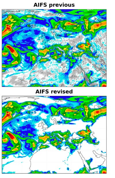
This hidden variable is an unexpected benefit, but I think we should be careful about generalizing the finding. The bounded variables are local expressions of large-scale conditions (e.g., precipitation in a region of large-scale ascent), so even if some information is thrown away by the bounding, the network still has lots of other relevant information. And these variables have short time-scales compared to the typical time step of a forecast (say 30 minutes versus 6 hours). Retaining memory may be less important for things like precipitation, local cloud cover, etc.
Finally, the network architecture is notable. By building the constraints directly into the network, you allow it to spontaneously adjust. In principle, the same bounds could be enforced in post-processing or through the loss function, but I suspect you get more benefit from telling the network something about the geometry of the problem and letting it take advantage of that information. Beucler et al. found a similar result when exploring different strategies for enforcing conservation laws in subgrid schemes in climate models, with hard-coding the conservation into the network’s final layers guaranteeing exact conservation without affecting skill, whereas loss function penalties produce only approximate conservation.
So these results suggest easy wins are available for variables that have clear physical bounds, short time-scales and are strongly tied to the large-scale state of the atmosphere. It may be a good idea to design forecast systems around such variables – using relative rather than specific humidity – wherever possible.
Global Constraints
Global constraints are harder to enforce. If a model doesn’t conserve energy, the modeler has to decide where to add or remove the extra energy. This is an old issue in climate/weather modeling, and most early climate models included flux corrections to account for model drift.
Sha et al. propose a simple fix of just rescaling three model variables – total water (qt), precipitation and temperature – to ensure they are conserved. This rescaling improves precipitation forecasts (including the drizzle problem) and large-scale features like 500hPa geopotential height, by 5-10% at longer lead-times.
The improvements are larger at longer lead times, which I think reflects the autoregressive rollout of ML forecasts. Because the forecast is generated autoregressively, small errors due to non-conservation compound, and anything that brings the system closer to the “true” path improves the forecast. The authors also note “performance gains likely propagate through cross-variable correlations” that the system learns. If you think the models have learned some physics, then improving temperature should improve geopotential forecasts.
The importance of getting the physics right means the adjustments have to be done in a specific order. First, negative humidity and precipitation values are zeroed out (bounded variables again). Then the total water is adjusted to conserve dry air mass and the precipitation is tuned to match the residual and close the moisture budget. Finally, the temperature is rescaled to close the total energy budget. Each adjustment fixes a quantity that the next budget depends on, so the corrections have to proceed sequentially. You have to understand the budgets to make the adjustments work.
There are some caveats, however. The network can become unstable early in training when the adjustments are large, so it’s best to start from a spun-up checkpoint. And the authors had to restrict the water adjustment to below 600 hPa to keep training stable, hinting that there may be more skill to squeeze out by optimizing the adjustments further. Finally, the surface fluxes (evaporation, radiative fluxes, etc.) see little improvement, since nothing corrects them directly.
This is a promising first pass, showing that simple approaches can work (at least in one ML system) provided they are guided by physics. It would be interesting to extend this approach to the momentum budget and to compare with other ways of enforcing conservation. Yuval and O’Gorman used a flux-form approach when parameterizing subgrid-scale fluxes in a climate model – predicting fluxes of a quantity between grid cells rather than the quantity itself (e.g., water vapor fluxes rather than total water vapor). Using the flux form is an old climate modeling trick, and guarantees conservation; whatever leaves one cell has to enter its neighbor. Similar to choosing bounded variables, it may be worth designing networks where the physics comes for free.
The Kinetic Energy Spectrum
So far we’ve discussed bounds and conservation laws, but there are other, more subtle, physical constraints that have been implemented. The atmosphere has a well-known kinetic energy (KE) spectrum, going from a k-3 slope at large scales (~geostrophic turbulence) to k-5/3 slope at small scales (~isotropic turbulence). This has been known since the 1980s, and reproducing it is a good test of whether a model’s flow “looks right”.
In practice, deterministic ML models struggle to reproduce these spectra due to the “blurring” problem: they produce overly smooth flows without enough energy at small scales. The reason for this is the MSE loss function, as I discussed in a previous post. So we shouldn’t expect deterministic models to reproduce the spectrum. FastNet tries to address this issue using a modified spherical harmonic (MSH) loss that penalizes spectral amplitude errors, producing slightly worse MSE scores, but improved spectral properties. This is what we’d expect – the blurring stops the models from being overconfident, at the expense of less realistic flow fields.
Probabilistic models can reproduce the spectra more faithfully by producing ensembles of forecasts. The ensemble-mean might be blurred, but each ensemble member can have reasonable spectral properties, via a diffusion objective in GenCast or a Continuous Ranked Probability Score loss in other models.

But a pointwise score only constrains each gridpoint’s distribution, not the larger spatial correlations. In practice, probabilistic models tend to have too much power at large wavenumbers (small scales). FourCastNet3 uses two tricks to improve this: (1) using spherical Fourier neural operators, rather than planar convolutions on a regular lat-lon grid, and (2) enforcing the CRPS loss at both the local and global distributions. It’s difficult to untangle the relative contributions of these fixes, but they seem to improve the small-scale energetics.
Lessons and Questions
Enforcing physical constraints has been less of a focus in ML WF models than in ML climate models. We want to run climate models for hundreds of years, so things like energy conservation are important for keeping the models stable. WF models are run for a few days or weeks, so it’s not as obvious that physical constraints need to be enforced. Nevertheless, the work so far is promising and gives some clear lessons for applying physical constraints to ML forecast models:
Physical constraints improve skill, not just model realism. In almost all the cases discussed here, enforcing physics made the forecasts better and often came with unexpected benefits.
The constraints work best when applied to the model’s forward pass, rather than through the loss-function or post-processing (as Beucler et al already showed for climate models). The networks take advantage of the extra information about the problem to produce unexpected benefits.
Adding bounding layers for all variables that have clear physical bounds seems like an easy win, and models should probably be designed to use bounded variables wherever possible.
Related: network design can make the constraints free. In addition to the bounded variables, using flux-form variables can give global conservation, and using spherical operators can improve energy spectra.
But there are also a number of open questions:
Does bounding generalize beyond precipitation, cloud cover, etc.? I suggested switching from specific to relative humidity, but it’s possible that this wouldn’t be as effective/stable.
How much of the gain from enforcing conservation survives once bounding is in place? It would be worth checking that global conservation leads to improvement when including bounded variables (e.g., the drizzle problem is already solved). Global conservation might add complexity without improving forecast skill.
What is the best enforcement route for global conservation: rescaling, flux-form or some kind of activation-layer constraint (if possible)? It would be informative to systematically compare these approaches.
And if we do rescaling, how much more tuning is needed? Sha et al had to implement the 600hPa cut-off and the correction ordering. Can we get more skill out of further tuning? And does each budget need to be tuned separately?
Do the hard constraints transfer on to the probabilistic approaches? I.e., can we both bound variables and use generative approaches?
Finally: what other constraints should we enforce? Presumably there is some frontier at which additional constraints add complexity without improving model performance. I suspect we aren’t there yet, but we should think carefully about the next constraints to add.
A final meta question is the most effective path forward. There is a hierarchy of constraints and enforcement mechanisms: bounding the variables requires an extra activation layer, closing the global budgets requires corrections in the training loop, and statistical constraints require new types of models. It’s tempting to work bottom-up (bounded variables to spectra), taking the easy wins first. But since the statistical constraints require the largest intervention, the best approach is probably top-down: first get the right system architecture and objective to satisfy the statistical constraints, then add variable bounding within that framework, and only then enforce global conservation, if it’s even still necessary.